1. Introduction
When you build your first trading dashboard, the data access pattern is usually wonderfully simple. You write a query like this:
SELECT
    symbol,
    SUM(quantity) AS total_volume
FROM trades
WHERE timestamp >= now() - interval '1 day'
GROUP BY symbol;
In the beginning, this works perfectly. Your PostgreSQL or MySQL database executes the query in a few milliseconds. Your dashboard loads instantly. Everyone is happy.
But what happens when your exchange grows?
Suddenly, your matching engine isn't producing ten trades a minute , it's producing thousands of trades a second. That simple SUM() query is now trying to scan through millions of rows every time a user refreshes their dashboard. The database CPU spikes, memory gets exhausted, and queries that used to take milliseconds now take minutes—or time out completely.
At this inflection point, you cannot simply add more RAM or tweak a B-Tree index. The fundamental reality of high-throughput systems is this: the architecture eventually changes, not just the SQL query.
Key Takeaway: Raw SQL queries on transactional data scale linearly with volume. To maintain constant-time performance, you must shift your architectural approach, not just your indexing strategy.
2. OLTP vs OLAP
Before diving into solutions, we need to understand the structural difference between recording events and analyzing them.
Databases generally fall into two broad categories: Online Transaction Processing (OLTP) and Online Analytical Processing (OLAP). They have entirely different optimization goals.
| Feature | OLTP (e.g., PostgreSQL, MySQL) | OLAP (e.g., ClickHouse, Redshift) |
|---|---|---|
| Purpose | Running the business (Transactions) | Understanding the business (Analytics) |
| Query Pattern | SELECT * WHERE id = 123 | SELECT SUM(x) GROUP BY y |
| Reads | Small, frequent, point-lookups | Massive, sweeping aggregations |
| Writes | Constant row-level inserts/updates | Large batch appends, rare updates |
| Storage Layout | Row-oriented | Column-oriented |
| Compression | Low (needs fast single-row writes) | Extremely High (repetitive column data) |
| Example Databases | PostgreSQL, MySQL, Oracle | ClickHouse, Snowflake, BigQuery |
| Example Workloads | User logins, Matching engines | Dashboards, Risk analysis, VWAP |
A trading engine (OLTP) needs to ensure that when Alice buys 1 BTC from Bob, the transaction is perfectly ACID compliant. An analytical dashboard (OLAP) doesn't care about the individual transaction, it only cares that the total volume for BTC increased by 1.
Key Takeaway: Transactional databases are optimized for safely writing single rows. Analytical databases are optimized for rapidly summarizing millions of rows.
3. Why Dashboards Become Slow
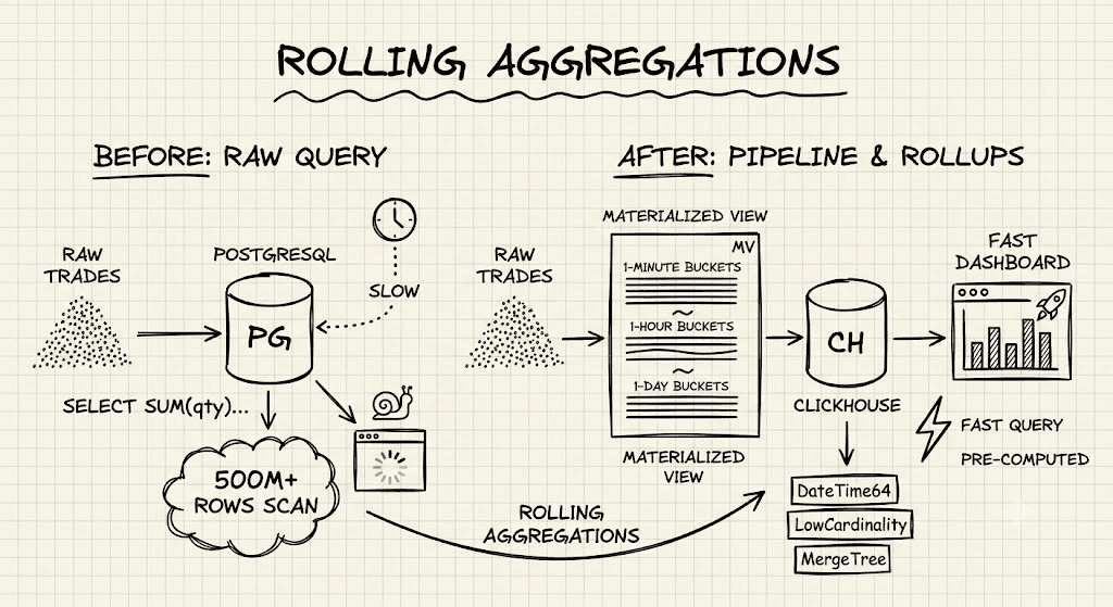
Imagine your exchange has processed 500 million trades today.
You have a live dashboard showing the 24-hour volume, grouped by symbol. When a user opens the dashboard, the following process occurs:
Every single time a user refreshes the page, the database repeats this exact same computation. It reads the same 500 million rows, recalculates the same sums, and sorts the same results.
If you add a standard B-Tree index on (timestamp, symbol), the database can find the starting point of the day faster. However, the database still has to physically scan all the rows that match the time range to compute the SUM(), COUNT(), or AVG().
Indexes are essentially sorted pointers. They tell the database where the data is, but they don't do the math for you. If you ask for the sum of 500 million numbers, the CPU still has to execute 500 million addition operations.
Key Takeaway: Traditional indexes speed up data retrieval, but they do not eliminate the CPU cost of computation. Repeatedly computing the same aggregations over raw data is the primary cause of dashboard degradation.
4. Introducing Rolling Aggregations
Production systems at scale stop asking raw questions. Instead, they continuously compute the answers ahead of time.
This concept is called rolling aggregations (or materialized rollups).
Instead of waiting for a user to request the 24-hour volume and then scanning 500 million trades, we chop time into manageable buckets. As raw trades flow in, we continuously aggregate them in the background into 1-minute blocks.
If a dashboard needs the 24-hour volume, it no longer looks at the trades table. It looks at the trades_1m aggregated table.
There are 1,440 minutes in a day. Even if you have 1,000 different trading pairs, scanning 1,440 rows per pair is dramatically cheaper and faster than scanning 500 million individual trades.
You are effectively trading a small amount of storage space (to store the aggregates) for a massive reduction in CPU usage and read latency at query time.
Key Takeaway: Rolling aggregations shift the computational burden from read-time (when the user is waiting) to write-time (when the data arrives).
5. Why Analytical Databases Exist
While you can build rolling aggregations in PostgreSQL using triggers or background cron jobs, it becomes painful at scale. PostgreSQL is inherently a row-store. Constant heavy writes and background re-computations cause MVCC (Multi-Version Concurrency Control) bloat, leading to massive table vacuuming overhead.
To support the workload of ingesting hundreds of thousands of events per second while simultaneously aggregating them, the database engines themselves had to evolve.
Analytical databases were built from the ground up under the assumption that data is immutable, queries touch specific columns across millions of rows, and aggregations are the primary workload.
Key Takeaway: We don't use analytical databases just because they are "fast." We use them because their physical storage architecture aligns perfectly with the mechanics of aggregating time-series data.
6. Time-Series Database Internals
To understand why a database like ClickHouse is so fast at these workloads, we have to look at how data is physically laid out on disk. Let's peel back the layers.
Write Ahead Log (WAL)
Writing directly to heavily compressed, sorted analytical tables is slow. To handle high-velocity inserts (like a firehose of market trades), databases first write incoming data to memory and append it to a Write Ahead Log (WAL) on disk for durability.
This guarantees data isn't lost if the server crashes, while allowing the database to batch rows together before performing expensive compression and sorting operations.
Row Storage vs Column Storage
In PostgreSQL (row store), a single trade is written to disk as a continuous block of bytes:
[TradeID, Timestamp, Symbol, Price, Quantity, Side]
If you run SELECT SUM(quantity), PostgreSQL must load the entire row from disk into memory, extract the quantity, and throw the rest away.
In ClickHouse (column store), columns are stored in separate files:
[TradeID, TradeID, TradeID]
[Quantity, Quantity, Quantity]
When you ask for SUM(quantity), ClickHouse only reads the file containing quantities. Disk I/O is the slowest part of a database, column stores minimize I/O by only reading the exact attributes requested.
Delta Encoding
Because column stores group identical data types together, compression algorithms become incredibly effective. Consider a timestamp column for high-frequency trades:
1712450101, 1712450102, 1712450103
Instead of storing the full 10-digit integer every time, the database stores the first value, and then only the difference (delta) between subsequent values:
1712450101, +1, +1
Suddenly, you are storing bytes instead of 64-bit integers.
Double Delta Encoding
If trades arrive at a perfectly consistent rate, the delta itself becomes constant (e.g., always +1). Double delta encoding stores the difference of the differences. If the deltas are +1, +1, +1, the double deltas become 0, 0, 0. A stream of zeros is exceptionally cheap to compress.
Dictionary Encoding
Market data has low cardinality fields. The symbol column might contain BTCUSDT ten million times a day. Storing a 7-byte string millions of times is wasteful.
Dictionary encoding maps strings to integers.
BTCUSDT = 1
ETHUSDT = 2
The database stores [1, 1, 1, 2] and translates it back to text only at the very end of the query execution. ClickHouse natively supports this via the LowCardinality(String) type.
Compression: LZ4 vs ZSTD
Once encoded, the data blocks are compressed. Databases usually offer a choice:
- LZ4: Blazing fast decompression. High CPU efficiency, moderate storage footprint. (Default in ClickHouse).
- ZSTD: Deep compression. Saves massive amounts of disk space but requires more CPU to uncompress during queries.
Sparse Indexes
B-Tree indexes (like in OLTP) keep a pointer for every single row. If you have a billion rows, the index is massive and must be paged into RAM.
Analytical databases use Sparse Indexes. Data is sorted by the primary key, and divided into "granules" (e.g., blocks of 8,192 rows). The index only stores the min and max value for each block.
Because the index is sparse, it is tiny. It easily fits entirely in CPU cache. It doesn't tell the database exactly where row #4,000,001 is, it tells the database "the row you want is somewhere inside block 500."
Data Skipping
Because of the sparse index, if you query WHERE timestamp > yesterday, the database looks at the min/max of the blocks. If a block's max timestamp is from last week, the engine drops the entire block instantly. It prunes out millions of rows without reading a single byte of their actual data from disk.
MergeTree
In ClickHouse, the core storage engine is called MergeTree. As data flushes from memory, it creates small, immutable "parts" on disk. In the background, ClickHouse constantly merges these smaller parts into larger, more heavily compressed parts (much like an LSM tree). This allows for rapid inserts while maintaining highly optimized read paths.
Key Takeaway: Analytical databases derive their speed not from a single magic trick, but from a coordinated architecture: column-oriented I/O, extreme compression, and sparse indexing that skips reading irrelevant data entirely.
7. Building A Fake Exchange
To prove these concepts, we need data. Not thousands of rows—millions. We'll write a small Python generator to simulate high-frequency trading data with realistic distributions (heavy concentration in BTC and ETH, rapid timestamps, realistic tick sizes).
import csv
import random
from datetime import datetime, timedelta

symbols = ['BTCUSDT'] * 65 + ['ETHUSDT'] * 20 + ['SOLUSDT'] * 10 + ['DOGEUSDT'] * 5
sides = ['BUY', 'SELL']
strategies = ['VWAP', 'TWAP', 'ARBITRAGE', 'RETAIL']

start_time = datetime.now() - timedelta(days=7)

with open('synthetic_trades.csv', 'w', newline='') as f:
    writer = csv.writer(f)
    for i in range(5_000_000): # Generate 5M rows for our test
        symbol = random.choice(symbols)
        price = round(random.uniform(10, 60000), 2)
        qty = round(random.uniform(0.001, 2.0), 4)

        writer.writerow([
            i,
            int(start_time.timestamp() * 1000),
            symbol, price, qty,
            random.choice(sides),
            random.choice(strategies),
            random.randint(5, 50) # latency in ms
        ])

        # Advance time by a few milliseconds
        start_time += timedelta(milliseconds=random.randint(1, 10))
Key Takeaway: Generating realistic synthetic data (with deliberate skew, like 65% BTC volume) is crucial for testing. If data is perfectly random, compression and dictionary encoding benchmarks will be highly inaccurate.
8. PostgreSQL Implementation
Let's see how standard PostgreSQL handles this.
CREATE TABLE pg_trades (
    trade_id BIGINT PRIMARY KEY,
    ts_millis BIGINT,
    symbol VARCHAR(16),
    price NUMERIC(12, 2),
    quantity NUMERIC(12, 4),
    side VARCHAR(4),
    strategy VARCHAR(16),
    latency_ms INT
);

-- Crucial for time-series lookups
CREATE INDEX idx_trades_time_sym ON pg_trades(ts_millis, symbol);
Let's run an analytical query: calculating the total volume and average latency for BTCUSDT over our dataset.
EXPLAIN ANALYZE
SELECT
    symbol,
    SUM(quantity) as total_vol,
    AVG(latency_ms) as avg_latency
FROM pg_trades
WHERE symbol = 'BTCUSDT'
GROUP BY symbol;
The PostgreSQL Execution Plan:
Even with the index, you will likely see a Bitmap Heap Scan followed by a HashAggregate. PostgreSQL uses the index to find all BTCUSDT rows, but it still has to fetch the actual table blocks (the Heap) to retrieve the quantity and latency_ms values.
If this query touches millions of rows, it will take several seconds. Worse, it evicts other useful data from the PostgreSQL shared_buffers cache, slowing down the rest of your OLTP workload.
Key Takeaway: PostgreSQL executes row-by-row. Even with perfect indexes, pulling specific columns out of millions of rows causes high I/O and cache pollution.
9. Moving To ClickHouse
Now, let's build the exact same table in ClickHouse. Notice how much more intentional the schema definition is.
CREATE TABLE ch_trades (
    trade_id UInt64,
    timestamp DateTime64(3), -- Millisecond precision
    symbol LowCardinality(String), -- Dictionary encoded!
    price Float64,
    quantity Float64,
    side LowCardinality(String),
    strategy LowCardinality(String),
    latency_ms UInt16 -- Smaller integer footprint
)
ENGINE = MergeTree()
PARTITION BY toYYYYMMDD(timestamp)
ORDER BY (symbol, timestamp);
Design Decisions:
DateTime64(3): Native millisecond type, highly compressible via double-delta.LowCardinality: Automatically applies dictionary encoding. String comparisons become extremely fast integer comparisons.PARTITION BY: Drops physical data files into daily buckets. A query for "today" entirely skips reading yesterday's folders on the filesystem.ORDER BY: This dictates the physical sort order on disk and defines the sparse index. Queries filtering bysymbolfirst, thentimestamp, will be lightning fast.
When we run the identical SUM() query in ClickHouse, it utilizes vectorized execution. Instead of processing one row at a time, ClickHouse loads a continuous block of thousands of memory-aligned quantity values and processes them in a single CPU instruction (SIMD). The query takes milliseconds.
Key Takeaway: In ClickHouse, the schema isn't just a data contract, it is a physical storage directive. How you define your types and
ORDER BYdictates your disk footprint and query speed.
10. Optimising ClickHouse: The AggregatingMergeTree
ClickHouse is fast at scanning raw data, but scanning raw data is still mathematically inferior to not scanning data at all.
This is where ClickHouse truly shines: native, background rolling aggregations using Materialized Views paired with an AggregatingMergeTree.
We want to pre-calculate the 1-minute volume and latency profiles as the data streams in.
Step 1: Create the destination table for our aggregates.
CREATE TABLE ch_trades_1m_aggs (
    window_start DateTime,
    symbol LowCardinality(String),
    total_trades AggregateFunction(count, UInt64),
    total_volume AggregateFunction(sum, Float64),
    avg_latency AggregateFunction(avg, UInt16)
)
ENGINE = AggregatingMergeTree()
ORDER BY (symbol, window_start);
(Notice the special AggregateFunction types. ClickHouse doesn't just store the final number; it stores the intermediate state required to combine multiple aggregates later).
Step 2: Create the Materialized View.
CREATE MATERIALIZED VIEW ch_trades_mv
TO ch_trades_1m_aggs AS
SELECT
    toStartOfMinute(timestamp) AS window_start,
    symbol,
    countState(trade_id) AS total_trades,
    sumState(quantity) AS total_volume,
    avgState(latency_ms) AS avg_latency
FROM ch_trades
GROUP BY window_start, symbol;
What happens now?
When you INSERT raw trades into ch_trades, ClickHouse intercepts the data block in memory, computes the 1-minute aggregations on the fly, and pushes the summarized results into ch_trades_1m_aggs.
To query it, you use the Merge suffix:
SELECT
    window_start,
    sumMerge(total_volume) as volume
FROM ch_trades_1m_aggs
GROUP BY window_start;
Your dashboard query just bypassed scanning 500 million rows. It scanned a few hundred aggregated rows. You achieved constant-time query latency regardless of market volume.
Key Takeaway: ClickHouse Materialized Views act as insert-triggers that build rolling aggregations asynchronously. They are the ultimate cheat code for high-performance dashboards.
11. Final Architecture
Putting it all together, a modern, resilient post-trade analytics pipeline looks like this:
- Trading Engine: Generates raw events.
- Kafka (Message Queue): Acts as the shock absorber. It buffers massive volume spikes and allows multiple systems to consume the same data independently.
- PostgreSQL: Handles the OLTP requirements (user balances, order states, ledger). It does not power the analytics dashboards.
- ClickHouse (Raw): Ingests the raw firehose for ad-hoc quant research and compliance auditing.
- ClickHouse (Aggregates): Automatically maintains the 1-minute, 1-hour, and 1-day rollups via Materialized Views.
- Dashboard API: Directly queries the rollups for sub-10ms UI rendering.
Key Takeaway: Decoupling the transactional ledger (PostgreSQL) from the analytical engine (ClickHouse) via a stream (Kafka) ensures that a spike in read queries never impacts the ability to match trades.
12. Conclusion
When your data footprint scales, the instinct is often to write cleverer SQL queries or spend hours tuning PostgreSQL configurations. While helpful, these are ultimately band-aids on a structural problem.
Performance engineering at scale isn't about making a heavy, millions-of-rows SQL query run 10% faster. It is about redesigning the architecture so that the expensive query no longer exists.
Analytical databases like ClickHouse give you the specialized physical storage to compress and scan raw data efficiently. But more importantly, through tools like the AggregatingMergeTree, they provide the framework to seamlessly implement rolling aggregations.
By calculating the answers as the data arrives, rather than when the user asks for it, you eliminate unnecessary computation. And in distributed systems, the fastest computation is the one you never have to perform.